Verifying Optimized Structures

Objective

The objective of this tutorial is to check if an optimized truncated model is consistent with the greater protein environment. This is useful for determining if the geometry of the optimized truncated model is feasible if the surrounding protein were present.

This workflow allows you to:

Compare the optimized structure with the original structure file.
Verify if the optimized structure is probable in the original structure file.

It is recommended to first visit the QM-only calculation workflow since the first half of the portion stems from it. You can find it here.

In this specific example, we are using ketosteroid isomerase (KSI) as the model system. The structure for KSI is obtained from the PDB 1OH0. In this PDB, KSI is bound to equilenin (EQU), which is an analogue of the dienolate reaction intermediate. Quite often, it is seen that resolved crystal structures contain non-reactive analogues; however, most QM studies aim to study the reaction path. Since our purpose is to examine the activity of KSI, we need to replace EQU with the intermediate analogue, 19NT, then reoptimize with our substrate, 5AND. Since EQU and 19NT are structural analogues, we can skip a complicated docking procedure and use QMzyme to align and replace EQU with 19NT, providing our reactive starting structure. When undergoing geometry optimizations, it is possible that the optimized structure might be in an orientation that clashes with the initial structure model. To resolve this, we need to identify if our optimized KSI structure with 19NT bound does not clash with the initial crystal structure.

In this tutorial, we will use a distance cutoff of 3 Å to undergo geometry optimization. Then, we will load our full environment from a model_cutoff_3.pkl file, import the optimized geometry output file, align them using C-alpha atoms, and examine if the resulting optimized structure is feasible.

Classes used in this example

Generate Model
QM_method
SelectionSchemes
DistanceCutoff SelectionSchemes (optional)
QMzymeRegion
- align_to method
CA_terminal TruncationSheme

Required Files

To start, you will need:

A fully prepped and protonated PDB.
An output file from geometry optimization.

[3]:

# Here are the necesary imports for this tutorial!

import QMzyme
from QMzyme import GenerateModel
from QMzyme.SelectionSchemes import DistanceCutoff
from QMzyme.data import PDB_xtal, LIG, OPT_C3
from QMzyme.RegionBuilder import RegionBuilder
import numpy as np
import QMzyme.MDAnalysisWrapper as MDAwrapper
from MDAnalysis.lib.distances import distance_array
import MDAnalysis

Preparing QM Input File for Optimization

Let’s start by creating an input file for optimization of 1oh0. For this, we will use the Molecule Replacement Using QMzyme workflow to first create the optimization input file! Specifically, we will be using a distance cutoff of 3 Å with our ligand replaced from EQU to 19NT. This section exists to demonstrate the process of making QM-input and .pkl files for the next section.

[ ]:

model = QMzyme.GenerateModel(PDB_xtal)
QMzyme.data.residue_charges.update({'EQU': -1}) # EQU ligand
model.set_catalytic_center(selection='resname EQU and segid A')
model.set_region(selection='resname EQU and segid A', name='old_ligand')
model.set_region(selection=DistanceCutoff, cutoff=3)

region_19nt = model.import_region(LIG, name='19nt')
QMzyme.data.residue_charges.update({'6VW': 0})
original_resid = model.old_ligand.atoms[0].resid
region_19nt.atom_group.residues.resids = original_resid
for atom in region_19nt.atoms:
    atom.resid = original_resid

region_19nt.align_to(other=model.old_ligand,
    self_selection="element C", other_selection="element C")

new_region = model.get_region("cutoff_3")
new_region = new_region.subtract(model.old_ligand)
new_region = new_region.combine(region_19nt)
model.set_region(selection=new_region, name=f"ksi_19nt_cutoff3")

ca_atoms = model.ksi_19nt_cutoff3.get_atoms(attribute="name", value="CA")
model.ksi_19nt_cutoff3.set_fixed_atoms(atoms=ca_atoms)

qm_method = QMzyme.QM_Method(
    basis_set='6-31G*',
    functional='wB97X-D3',
    qm_input='OPT FREQ',
    program='gaussian'
)
qm_method.assign_to_region(region=model.ksi_19nt_cutoff3)

model.truncate()
model.write_input()

Loading Pickled QMzymeModel

After running the geometry optimization, it is always important to validate your resulting structures! To do this, we will load our original full-system using the .pkl file from input file generation. Because quantum chemistry software can sometimes alter atom naming conventions or strip residue metadata, we run a quick loop to map the original names, IDs, and residue labels from our reference model directly onto our optimized atoms. This ensures everything matches perfectly before we align the structures.

[5]:

model = QMzyme.GenerateModel(pickle_file='1oh0_equ_crystal.pkl')
universe_opt = MDAnalysis.Universe(OPT_C3)
region_opt = RegionBuilder(name='opt', atom_group=universe_opt.select_atoms("all")).get_region()
ref_region = model.get_region("ksi_19nt_cutoff3_truncated")

for opt_atom, ref_atom in zip(region_opt.atoms, ref_region.atoms):
    opt_atom.name = ref_atom.name
    opt_atom.resid = ref_atom.resid
    opt_atom.resname = ref_atom.resname

Aligning C-alpha Atoms of Original and Optimized Structuresd

The align_to() method is present in the QMzymeRegion class. It can be used to align specific atoms and then update the aligned atoms to the region.The alignment procedure also reports RMSD values before and after alignment.

⚠ Important considerations:

Align the substrate (self) to the full protein–ligand complex (other).
Do not align the other way around.
This can be ensured by specifying the substrate model before the “align_to” function. This will assign the substrate model to “self”.

This ensures:

The substrate region is updated to match the aligned coordinates.
The substrate moves into the position of the bound ligand.
The ligand does not move to the substrate coordinates.

Two critical arguments self_selection= and other_selection= specify the atoms used for alignment. Make sure that the number of atoms in the reference (self) and in the target (other) are the same. If the number of atoms in the selections differs, then the alignment will fail.

If your substrate PDB was generated independently (not modified directly from the bound ligand), ensure that corresponding heavy atoms are properly labeled. This will ensure that the correct atoms are getting aligned.

[6]:

# Now that region_opt knows which atoms are "CA", you can align them.
# Note: The standard MDAnalysis selection string for alpha carbons is "name CA"
region_opt.align_to(
    other=ref_region,
    self_selection="name CA",
    other_selection="name CA"
)

model.set_region(selection=region_opt, name="OPT_aligned")
model.set_region(selection="all", name="full_region")

RMSD before alignment: 72.48750305175781 \u00C5
RMSD after alignment: 4.2482093698830376e-05 \u00C5

Identifying Potential Clasing Residues

Now that our optimized geometry is aligned with the full system, we can examine if the optimized structure is feasible with the initial structure! To do this, we use the find_nearby_residues() method to compare our aligned, optimized region against the surrounding protein environment. The method calculates the distance between every atom in our optimized model (self) and every atom in the rest of the protein (other), skipping over identical residues. Any residue from the greater environment that falls within our 1.0 Å threshold will be flagged and printed out, showing you exactly which parts of the protein matrix would experience a severe steric clash due to the geometry optimization.

[7]:

# Call the method to find any residues in the full region
# that is within 1.0 Å from aligned optimized model.
model.OPT_aligned.find_nearby_residues(model.full_region, 1.0)

<QMzymeResidue resname: ILE, resid: 28, chain: X> is within 1.0 Å of <QMzymeResidue resname: TYR, resid: 16, chain: A>
<QMzymeResidue resname: ILE, resid: 102, chain: X> is within 1.0 Å of <QMzymeResidue resname: VAL, resid: 101, chain: A>
<QMzymeResidue resname: GLN, resid: 117, chain: X> is within 1.0 Å of <QMzymeResidue resname: MET, resid: 116, chain: A>

[7]:

[<QMzymeResidue resname: ILE, resid: 28, chain: X>,
 <QMzymeResidue resname: ILE, resid: 102, chain: X>,
 <QMzymeResidue resname: GLN, resid: 117, chain: X>]

Visualizing Clashing Residues

From this, we acquire three potential clashing pairs of residues. However, we cannot assume that residues are clashing from this information only. Thus, to examine how close they are, we will use pymol_visualize() to see how close these residues are. This is done by visualizing the overlay of OPT_aligned region with clashing_residues region.

[ ]:

# First create a region consisting of the clashing residues.
model.set_region(selection="resid 28 or resid 102 or resid 117", name="clashing_residues")

# Create pymol visualization.
model.pymol_visualize()

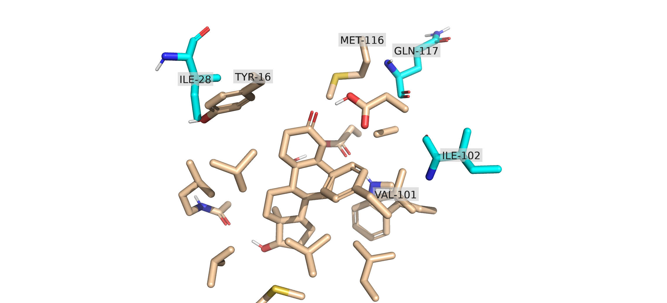
de63d7eee45e4fbaa1a5627a6cfed919

When you open the combined clashing_region in PyMOL, the spatial overlap between the full protein environment and your optimized model becomes visually striking. The bulky aromatic ring of TYR 16 has rotated or shifted during the quantum chemical optimization directly into the space occupied by the side chain of ILE 28. From this, we can conclude that the optimized structure is not structurally possible within the original protein structure.

References Cited

The PyMOL Molecular Graphics System, Version 3.0 Schrödinger, LLC.